首先选取沪深股票市场,本人比较关注的12只股票:
000002 万科A,600566 济川药业,300051 三五互联,002039 黔源电力,600872 中炬高新,300324 旋极信息,600885 宏发股份,600382 广东明珠,000732 泰和集团,002174 游族网络,000915 山大华特,002415 海康威视
备注: 如果是基金经理,则会有研究部门推荐的股票选择池
程序运行的得到结论如下:
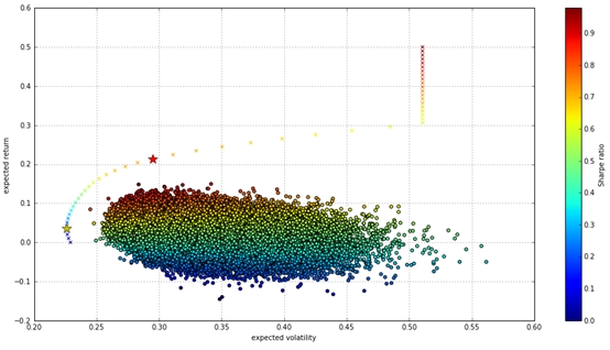
1. 当投资组合的sharpe值最大时,投资组合为:
41.2%的万科A,10.5%的广东明珠,38.2%的山大华特,10.1%的海康威视
该组合的未来预期年化收益为:21.4%
该组合的预期年化波动率为:29.5%
该组合的sharpe指数为0.725
2. 当投资组合的波动最小时,投资组合为:
34.5%的万科A,17.9%的济川药业,24.6%的黔源电力,2%的旋极信息,1%的宏发股份,9.4%的泰和集团,0.8%的游族网络,9.8%的海康威视
该组合的未来预期年化收益为:3.7%
该组合的预期年化波动率为:22.6%
该组合的sharpe指数为0.163
相关输出图表如下:
图1:关注的12只股票从2016-01-01到2016-12-01的归一化股价走势
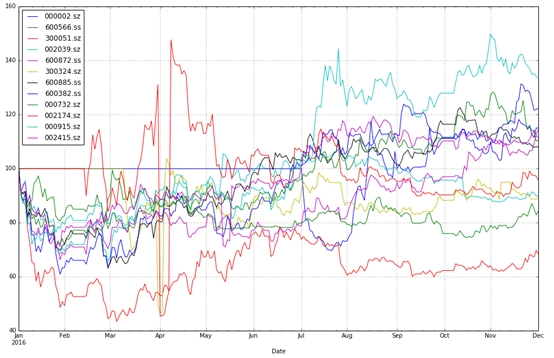
图2:10万次蒙特卡洛模拟计算,得到各种投资组合以及相应收益率和波动率
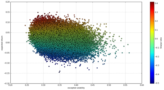
图3:有效前沿、最优投资组合的图
#叉号:构成的曲线是有效前沿(efficient frontier,目标收益率下最优的投资组合)
#红星:夏普值最大的投资组合
#黄星:方差最小的投资组合
程序源代码以及详细注释说明如下:
# -*- coding: utf-8 -*-
"""
Created on Thu Dec 8 01:26:52 2016
@author: Administrator
"""
import pandas as pd
import numpy as np
#import statsmodels.api as sm #统计运算
#import scipy.stats as scs #科学计算
import matplotlib.pyplot as plt #绘图
import pandas.io.data as web
#import tushare as ts
# 1.选取感兴趣的股票
# 000002 万科A,600566 济川药业,300051 三五互联,002039 黔源电力,600872 中炬高新,300324 旋极信息,600885 宏发股份,600382 广东明珠,000732 泰和集团,002174 游族网络,000915 山大华特,002415 海康威视
# 并比较一下数据(2016-01-01至2016-12-01)
symbols = ['000002.sz','600566.ss','300051.sz','002039.sz','600872.ss','300324.sz',
'600885.ss','600382.ss','000732.sz','002174.sz','000915.sz','002415.sz']
noa = len(symbols)
data = pd.DataFrame()
for sym in symbols:
data[sym] = web.DataReader(sym, data_source='yahoo',start='2016-01-01',
end='2016-12-01')['Adj Close']
data.columns = symbols
data.head(5)
(data / data.ix[0] * 100).plot(figsize=(16, 10), grid=True)
#2.计算不同证券的均值、协方差
#每年252个交易日,用每日收益得到年化收益。计算投资资产的协方差是构建资产组合过程的核心部分。运用pandas内置方法生产协方差矩阵。
returns = np.log(data / data.shift(1))
returns.mean()*252
returns.cov()*252
#3.给不同资产随机分配初始权重
#由于A股不允许建立空头头寸,所有的权重系数均在0-1之间
weights = np.random.random(noa)
weights /= np.sum(weights)
weights
# 4.计算预期组合年化收益、组合方差和组合标准差
np.sum(returns.mean()*weights)*252
np.dot(weights.T, np.dot(returns.cov()*252,weights))
np.sqrt(np.dot(weights.T, np.dot(returns.cov()* 252,weights)))
# 5.用蒙特卡洛模拟产生大量随机组合
#进行到此,我们最想知道的是给定的一个股票池(证券组合)如何找到风险和收益平衡的位置。
#下面通过一次蒙特卡洛模拟,产生大量随机的权重向量,并记录随机组合的预期收益和方差。
port_returns = []
port_variance = []
for p in range(100000):
weights = np.random.random(noa)
weights /=np.sum(weights)
port_returns.append(np.sum(returns.mean()*252*weights))
port_variance.append(np.sqrt(np.dot(weights.T, np.dot(returns.cov()*252, weights))))
port_returns = np.array(port_returns)
port_variance = np.array(port_variance)
#无风险利率设定为3%
risk_free = 0.03
plt.figure(figsize = (16,8))
plt.scatter(port_variance, port_returns, c=(port_returns-risk_free)/port_variance, marker = 'o')
plt.grid(True)
plt.xlabel('excepted volatility')
plt.ylabel('expected return')
plt.colorbar(label = 'Sharpe ratio')
#6.投资组合优化1——sharpe最大
#建立statistics函数来记录重要的投资组合统计数据(收益,方差和夏普比)
#通过对约束最优问题的求解,得到最优解。其中约束是权重总和为1。
def statistics(weights):
weights = np.array(weights)
port_returns = np.sum(returns.mean()*weights)*252
port_variance = np.sqrt(np.dot(weights.T, np.dot(returns.cov()*252,weights)))
return np.array([port_returns, port_variance, port_returns/port_variance])
#最优化投资组合的推导是一个约束最优化问题
import scipy.optimize as sco
#最小化夏普指数的负值
def min_sharpe(weights):
return -statistics(weights)[2]
#约束是所有参数(权重)的总和为1。这可以用minimize函数的约定表达如下
cons = ({'type':'eq', 'fun':lambda x: np.sum(x)-1})
#我们还将参数值(权重)限制在0和1之间。这些值以多个元组组成的一个元组形式提供给最小化函数
bnds = tuple((0,1) for x in range(noa))
#优化函数调用中忽略的唯一输入是起始参数列表(对权重的初始猜测)。我们简单的使用平均分布。
opts = sco.minimize(min_sharpe, noa*[1./noa,], method = 'SLSQP', bounds = bnds, constraints = cons)
opts
#得到的最优组合权重向量为:
opts['x'].round(3)
#sharpe最大的组合3个统计数据分别为:
#预期收益率、预期波动率、最优夏普指数
statistics(opts['x']).round(3)
#7.投资组合优化2——方差最小
#接下来,我们通过方差最小来选出最优投资组合。
#但是我们定义一个函数对 方差进行最小化
def min_variance(weights):
return statistics(weights)[1]
optv = sco.minimize(min_variance, noa*[1./noa,],method = 'SLSQP', bounds = bnds, constraints = cons)
optv
#方差最小的最优组合权重向量及组合的统计数据分别为:
optv['x'].round(3)
#得到的预期收益率、波动率和夏普指数
statistics(optv['x']).round(3)
#8.组合的有效前沿
#有效前沿有既定的目标收益率下方差最小的投资组合构成。
#在最优化时采用两个约束,1.给定目标收益率,2.投资组合权重和为1。
def min_variance(weights):
return statistics(weights)[1]
#在不同目标收益率水平(target_returns)循环时,最小化的一个约束条件会变化。
target_returns = np.linspace(0.0,0.5,50)
target_variance = []
for tar in target_returns:
cons = ({'type':'eq','fun':lambda x:statistics(x)[0]-tar},{'type':'eq','fun':lambda x:np.sum(x)-1})
res = sco.minimize(min_variance, noa*[1./noa,],method = 'SLSQP', bounds = bnds, constraints = cons)
target_variance.append(res['fun'])
target_variance = np.array(target_variance)
len(target_variance)
#下面是最优化结果的展示。
#叉号:构成的曲线是有效前沿(目标收益率下最优的投资组合)
#红星:sharpe最大的投资组合
#黄星:方差最小的投资组合
plt.figure(figsize = (16,8))
#圆圈:蒙特卡洛随机产生的组合分布
plt.scatter(port_variance, port_returns, c = port_returns/port_variance,marker = 'o')
#叉号:有效前沿
len(target_variance),len(target_returns)
plt.scatter(target_variance,target_returns, c = target_returns/target_variance, marker = 'x')
#红星:标记最高sharpe组合
plt.plot(statistics(opts['x'])[1], statistics(opts['x'])[0], 'r*', markersize = 15.0)
#黄星:标记最小方差组合
plt.plot(statistics(optv['x'])[1], statistics(optv['x'])[0], 'y*', markersize = 15.0)
plt.grid(True)
plt.xlabel('expected volatility')
plt.ylabel('expected return')
plt.colorbar(label = 'Sharpe ratio')
·END·